Test-Time Compute
Test-time compute as a second scaling axis. The three levers—more steps, more candidates and more structure—and their quality, cost and latency tradeoffs in reasoning models.
Links containing ?t= open the video at a specific second.
The ideas to retain
1. What test-time compute is and why it matters
For a long time, the main known lever for improving an LLM was training scale: more parameters, more data and more training compute. The original scaling-law work (Kaplan et al., 2020)…
2. The three levers
There are three principal mechanisms for translating additional inference compute into better answers.
Lever 1: More internal steps
Chain-of-thought (Wei et al., 2022) is the most direct mechanism. Instead of producing the final answer immediately, the model first generates a sequence of intermediate steps that…
Video text and visual description
This video has no speech. The text track reproduces the written content; the descriptions below explain the visuals.
0:00 — Test-Time Compute: the second scaling dimension.
The second scaling dimension. More steps. More candidates. Better compute decisions.
Visual description: Three mechanisms, sequential, parallel and structured, are revealed progressively to introduce three ways to spend more compute during inference.
0:09 — Not only train more. Think longer.
One lever is training: more parameters, more data and more compute to build the model. Kaplan's scaling laws documented that relationship in 2020. But there is a second dimension. How much compute is spent on each individual answer. That is test-time compute.
Visual description: Two columns separate training from inference and show that per-answer budget is distinct from the compute used to build model weights.
0:26 — Force the model to keep thinking.
Chain-of-thought decomposes a problem into intermediate steps. Reasoning models can extend that process. A technique called budget forcing suppresses the end token and adds "Wait". In the s1-32B study, budget forcing raised AIME24 from 50% to about 57%. More steps can improve an answer; they do not guarantee it.
Visual description: A Frame → Split → Check sequence is extended with Wait before the end token and ends with the reported AIME24 comparison, 50% → about 57%.
0:46 — Generate many answers. Keep the best.
Best-of-N generates several answers and uses an evaluator to select the best one. Another strategy is majority voting. The selection criterion matters as much as the number of candidates. On AIME 2024, o1 went from 74% with one sample to 83% with consensus across 64 samples. That is majority-based selection.
Visual description: Four candidates for 17 × 6 are evaluated and voted on; the screen then shows the reported o1 AIME 2024 comparison, 74% for one sample and 83% with consensus across 64 samples.
1:09 — Explore branches. Prune weak ones.
Tree search does not generate a single linear chain. It explores multiple branches, evaluates each one and prunes the least promising. Cost depends on how many branches are expanded. For complex planning, it lets the system compare alternative routes before continuing. Improvement is not automatic: it depends on the task, evaluator and search budget.
Visual description: A tree starts at the problem, expands routes A/B/C, prunes branches and keeps a selected route through Continue to illustrate exploration, evaluation and pruning.
1:29 — Each token waits for the previous one.
In standard autoregressive decoding, each token depends on the tokens before it. At a fixed rate of 100 tokens per second, generating a 5,000-token chain takes 50 seconds. Shortening the chain or generating tokens faster reduces that wait. The sequential dependency remains. Latency is a real design constraint.
Visual description: A row of tokens accumulates sequentially while a timeline ends in the illustrative calculation 5,000 ÷ 100 = 50 s.
1:49 — Larger model or more time to think.
Test-time compute and pretraining are complementary. On some tasks, a smaller model with more inference compute can outperform a larger model with less. Cost is no longer determined by size alone. Efficient systems adapt both the model and the budget to each problem. That decision requires task-level evaluation. That is complementary scaling.
Visual description: A plane compares model size with compute per query, placing a smaller model with more inference beside a larger model to explain complementary allocation.